Bibliometrix
Nikita Gusarov
Since the start of my Doctoral studies I’ve always performed the literature exploration “the hard way”. Meaning, that I’ve performed most of my literature searches by hand, attempting to manually locate the key articles in the domain. While I’ve got an in-depth comprehension of the field, it remains possible that I’ve overlooked some of interesting literature clusters. However, there always existed a possibility to avoid such mistakes: by performing a thorough bibliometrics study instead of the simple literature overview.
In this post I’ll present one of the known to me bibliometrics tools and solutions: the bibliometrix R package.
Evidently there exist stand-alone applications for bibliometrics studies, such as VOSviewer or inbuilt toolset of Lens.org or SCOPUS.
Nevertheless, I believe that having a tool which may be integrated directly within the workflow (ex: redaction of .Rmd documents) is extremely useful.
Setup
First of all we start with configuration of our workspace.
I adore the functionalities of the tidyverse.
The bibliometrix is required for demonstration of its capabilities.
# Package names
packages = c("tidyverse", "bibliometrix")

# Get installed packages
installed_packages = packages %in% rownames(installed.packages())
# Install if not installed
if (any(installed_packages == FALSE)) {
  install.packages(packages[!installed_packages])
}

# Load packages
invisible(
    lapply(packages, library, character.only = TRUE)
)
Once the packages installed and loaded, we should
The bibliometrix package relies on the convert2df() function for data interpretation.
This function takes as input one of the following:
- Clarivate Analytics WoS (in plaintext ‘.txt’, Endnote Desktop ‘.ciw’, or bibtex formats ‘.bib’);
- SCOPUS (exclusively in bibtex format ‘.bib’);
- Digital Science Dimensions (in csv ‘.csv’ or excel ‘.xlsx’ formats);
- Lens.org (in csv ‘.csv’);
- an object of the class pubmedR (package pubmedR) containing a collection obtained from a query performed with pubmedR package;
- an object of the class dimensionsR (package dimensionsR) containing a collection obtained from a query performed with dimensionsR package.
The other two arguments taken by the function are (1) the declaration of database source and (2) specification of filetype for certain databases.
The first one is dbsource, which should correspond to the database source as above:
wosscopusdimensionslensisipubmed
The second, format declares the format of the SCOPUS and Clarivate Analytics WoS export file:
apibibtexplaintextendnotecsvexcel
The resulting output is a unified database suited for further analysis. In other words this function mitigates the differences between all the available bibliography analysis providers. The output includes information about:
| Key | Value |
|---|---|
| AU | Authors |
| TI | Document Title |
| SO | Publication Name (or Source) |
| JI | ISO Source Abbreviation |
| DT | Document Type |
| DE | Authors’ Keywords |
| ID | Keywords associated by SCOPUS or WoS database |
| AB | Abstract |
| C1 | Author Address |
| RP | Reprint Address |
| CR | Cited References |
| TC | Times Cited |
| PY | Year |
| SC | Subject Category |
| UT | Unique Article Identifier |
| DB | Database |
For example, imagine we want to import dataset generated with WoS interface under .bib file format.
Here we use a simple dataset extracted from Web of Science.
For its generation we have used the following search pattern applied to all fields for all time:
(“econometrics” OR “Econometrics” OR “econometric” OR “econometrica”) AND (“machine learning” OR “Machine Learning”)
This can be achieved with the command:
# Convert database
db = convert2df(
    "wos.bib",
    dbsource = "wos",
    format = "bibtex"
)
Unfortunately, the documentation available on CRAN is partially outdated, because the project is still under active development. Th ebest source for documentation, features lookup, etc. is the official website of the initiative.
Some observations: - “lens” format has some problems with citations retrieval - “wos” and “scopus” are the two most developped formats
Simple bibliometric analysis
We may want to filter our results. For example, we may decide to exclude from our analysis such productions as: reviews, meeting abstracts, letters, editorial materials and corrections (as well as proceedings). Or simply select only the entries containing the article keyword:
db = db %>%
    filter(
        str_detect(
            DT, "ARTICLE"
        )
    )
The analysis may then be performed on the resulting database using the inbuilt toolset of the package.
The resulting object may be synthetysed using the inbuilt traditional R methods like summary() for example.
One of the problems of the methods’ implementation is the fact that it immediately prints the output.
# Analyse results
results = db %>%
    biblioAnalysis() %>%
    summary(
        k = 10,
        pause = F,
        width = 75
    )
The dataset covers the period from 1992 to 2022 (nowadays), containing only 278 articles (obviously, we have had them filtered) from 175 different sources (journals). Observing the number of authors and keywords in the database we can easily imagine the complexity of the analysis task.
As you can guess, this function performs all the required analysis automatically and provides the descriptive statistics of particular interest.
Evidently, we can as easy perform the same analysis by hand over the db database (or extract the results from results object), but the package offers quite handy alternative.
For example, we may want to get the main descriptive statistics, we can run:
# Output main
cat(results$MainInformation)
##
##
## MAIN INFORMATION ABOUT DATA
##
## Timespan 1992 : 2022
## Sources (Journals, Books, etc) 175
## Documents 278
## Average years from publication 3.2
## Average citations per documents 16.45
## Average citations per year per doc 2.988
## References 13361
##
## DOCUMENT TYPES
## article 233
## article; book chapter 8
## article; data paper 2
## article; early access 24
## article; proceedings paper 11
##
## DOCUMENT CONTENTS
## Keywords Plus (ID) 862
## Author's Keywords (DE) 1166
##
## AUTHORS
## Authors 736
## Author Appearances 847
## Authors of single-authored documents 26
## Authors of multi-authored documents 710
##
## AUTHORS COLLABORATION
## Single-authored documents 26
## Documents per Author 0.378
## Authors per Document 2.65
## Co-Authors per Documents 3.05
## Collaboration Index 2.82
## Another implmeentation of the standart method is plot() function:
plt = db %>%
    biblioAnalysis() %>%
    plot(results, k = 5, plot = FALSE)
The resulting plot object has the same inconveniences, as it attempts to store several plots inside one object, without supressing corresponding output. Here we call one of the plots - number of publications by year:
plot(plt$AnnualScientProd)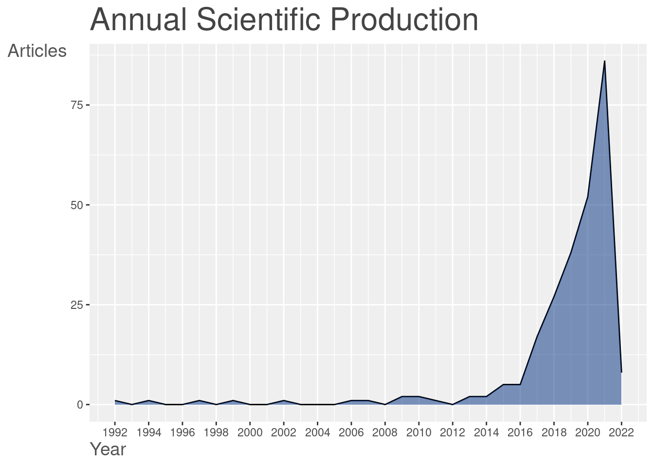
We see, that the idea of merging both econometrics and machine learning (ML) is fairly recent. The number of publications mentioning both econometrics and ML is extremely low at start of the century, plummeting recently (around 2016 - 2018). We may imagine that such tendency is due to the propagation of the ML toolset to the other disciplines. It is exactly the period where the ML becomes accessible enough for someone without Computer Science (CS) background to be tested in scientific studies.
Finally, there exist some auxiliary functions to enhance the basic analysis. To extract the most cited papers one can use1:
# Parse the cited
db_cite = citations(
    db, field = "article", sep = ";"
)

# Output the results
cbind(db_cite$Cited[1:10]) %>% knitr::kable()| BREIMAN L, 2001, MACH LEARN, V45, P5, DOI 10.1023/A:1010933404324 | 42 |
| TIBSHIRANI R, 1996, J ROY STAT SOC B MET, V58, P267, DOI 10.1111/J.2517-6161.1996.TB02080.X | 37 |
| VARIAN HR, 2014, J ECON PERSPECT, V28, P3, DOI 10.1257/JEP.28.2.3 | 23 |
| CORTES C, 1995, MACH LEARN, V20, P273, DOI 10.1007/BF00994018 | 21 |
| MULLAINATHAN S, 2017, J ECON PERSPECT, V31, P87, DOI 10.1257/JEP.31.2.87 | 21 |
| FRIEDMAN JH, 2001, ANN STAT, V29, P1189, DOI 10.1214/AOS/1013203451 | 20 |
| ZOU H, 2005, J R STAT SOC B, V67, P301, DOI 10.1111/J.1467-9868.2005.00503.X | 20 |
| BELLONI A, 2014, REV ECON STUD, V81, P608, DOI 10.1093/RESTUD/RDT044 | 18 |
| HASTIE T, 2009, ELEMENTS STAT LEARNI, DOI 10.1007/978-0-387-84858-7., 10.1007/978-0-387-84858-7 | 18 |
| ATHEY S, 2016, P NATL ACAD SCI USA, V113, P7353, DOI 10.1073/PNAS.1510489113 | 16 |
Keep in mind that the articles listed here are associated with the number of citations within the dataset. Obviously, such works as the article of Breiman L. (2001) is far more cited than this. The same applies to the work of Tibshirani (1996), which is quite popular in econometrics field.
Co-citation networks analysis
Speaking about more complex bibliometrics analysis we can mention several representations.
Firstly, we may trace the co-citation network, which demonstrates relations between cited references nodes. We provide the code to get summary descriptives for the generated network as well.
# We construct network and plot it
plt_cocit = db %>%
    biblioNetwork(
        analysis = "co-citation",
        network = "references",
        sep = ";"
    ) %>%
    networkPlot(
        n = 30, Title = "Co-Citation Network",
        remove.multiple = FALSE,
        remove.isolates = TRUE,
        type = "auto", # "fruchterman", "circle"
        size.cex = TRUE, size = 20,
        labelsize = 1,
        edgesize = 10, edges.min = 5
    )
# Plot
plot(plt_cocit$graph)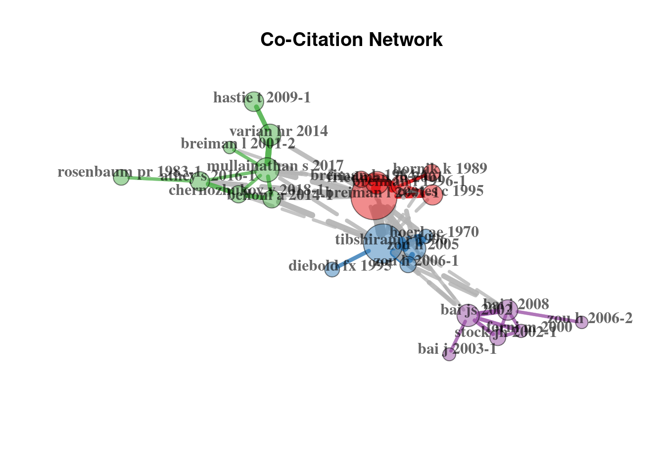
Secondly, we can observe the journal co-citation network, which is constructed by taking the journals as nodes.
# We construct network
plt_cocit_j = db %>%
    metaTagExtraction(
        "CR_SO",
        sep = ";"
    ) %>%
    biblioNetwork(
        analysis = "co-citation",
        network = "sources",
        sep = ";"
    ) %>%
    networkPlot(
        n = 20, remove.multiple = FALSE,
        Title = "Co-Citation Network",
        type = "auto",
        size.cex = TRUE, size = 15,
        labelsize = 1,
        edgesize = 10, edges.min = 5
    )
# Plot
plot(plt_cocit_j$graph)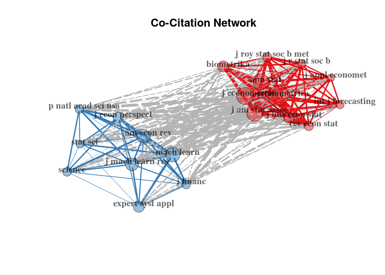
Here we distinguish two clusters: (1) one oriented on the econometrics, applied econometrics and statistical journals; and (2) another focusing on the ML methodology and natural sciences (where the ML toolset became more eagerly accepted than in the Economics domain).
Directed graphs for history tracking
With directed graphs we can depict the historical trends in citations and works interdependence, in terms of influence.
# Here we take upper 25% of citations
histgraph = db %>%
    histNetwork(
        min.citations = quantile(db$TC, 0.90),
        sep = ";"
    ) %>%
    histPlot(
        n = 40,
        size = 5,
        labelsize = 4
    )
# Plot
plot(histgraph$g)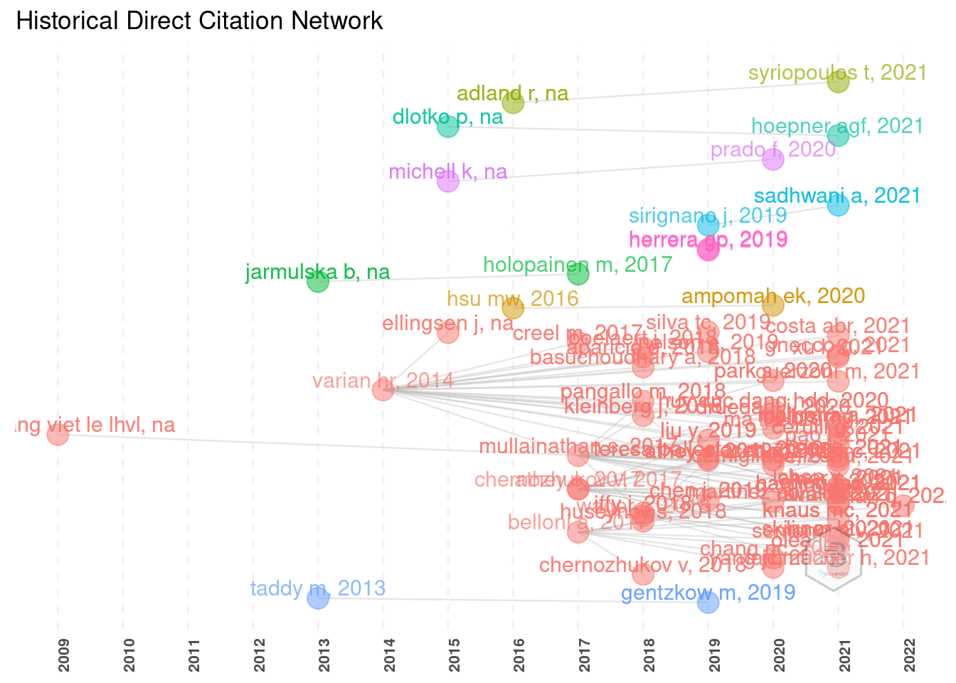
The outputs are sometimes extremely messy and require manual adjustment and tweaks.
For better readability it is possible to reduce the number of displayed entries, reduce the size of labels, etc.
Here one will have to be creative to fit such plot in a plain .pdf page.
Keywords analysis
Another stage is the keyword analysis, which can provide even more insight into the popular trends present in the given field.
As we discover the definition on the bibliometrix website:
Co-word networks show the conceptual structure, that uncovers links between concepts through term co-occurrences. Conceptual structure is often used to understand the topics covered by scholars (so-called research front) and identify what are the most important and the most recent issues. Dividing the whole timespan in different time-slices and comparing the conceptual structures is useful to analyse the evolution of topics over time.
Such type of bibliometric analysis may be performed with different tools.
The keyword co-occurrences exploration:
# Analysis
network = db %>%
    biblioNetwork(
        analysis = "co-occurrences",
        network = "keywords", sep = ";"
    ) %>%
    networkPlot(
        normalize = "association", n = 20,
        Title = "Keyword Co-occurrences",
        type = "fruchterman",
        size.cex = TRUE, size = 30,
        remove.multiple = FALSE,
        edgesize = 10, edges.min = 2,
        labelsize = 3, label.cex = TRUE, label.n = 30
    )
# Analysis
plot(network$graph)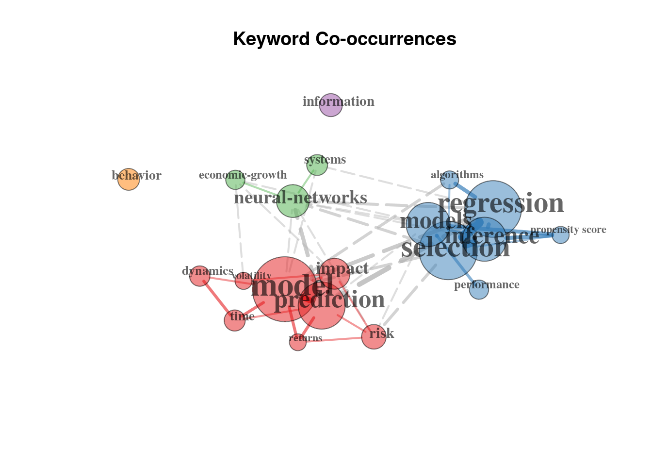
Which outlines three main clusters focused on (1) prediction, risks and time series related questions in context of ML; (2) the neural networks and (3) the regression analysis more traditional for econometrics, focused on inference and underlying models.
Another option is the Correspondence Analysis (CA). With it we may extract more information, among which the conceptual structure map and factorial map (ex: of the documents with the highest contributes).
plt_ca = conceptualStructure(
    db, method = "CA",
    field = "ID",
    minDegree = 10, k.max = 8,
    stemming = FALSE, labelsize = 8,
    documents = 10
)
# Conceptual structure map
plot(plt_ca$graph_terms)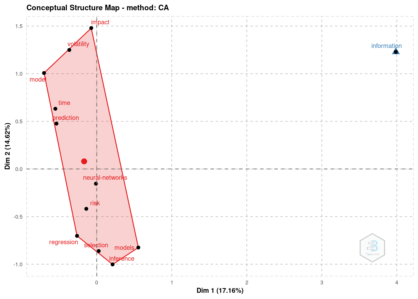
# Factorial map of the documents with the highest contributes
plot(plt_ca$graph_documents_Contrib)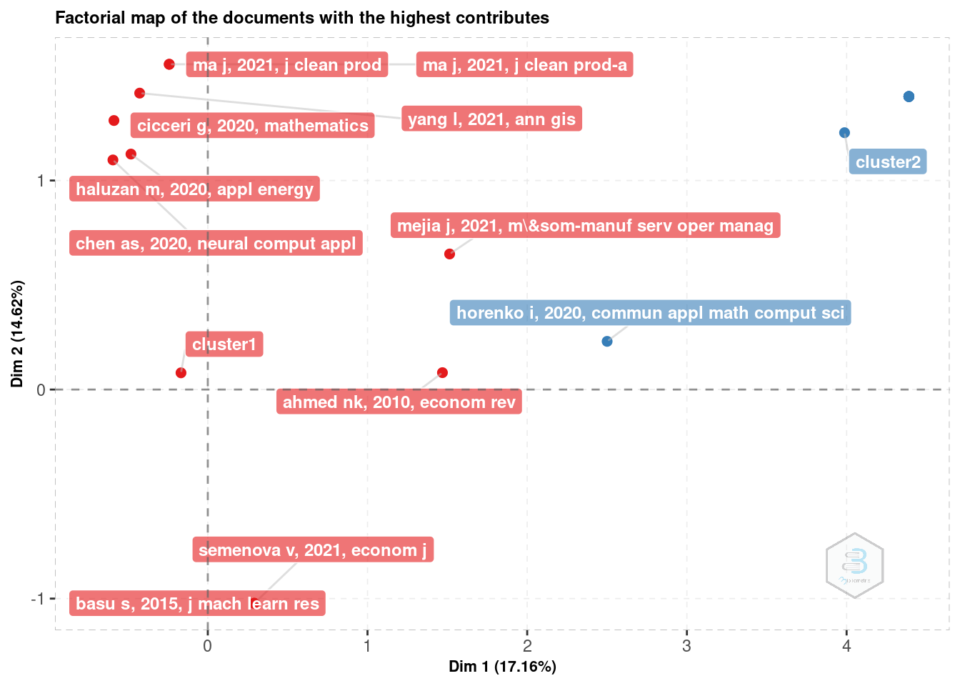
Before this data may be analysed it requires some tweaks and adjustments to the clustering algorithm, because otherwise it does not bring enough insight into the data.
At this point it is important to remember, that clustering techniques may not be completely reproducible between executions. One should always pay attention when using such automated algorithms for data analysis.
Collaboration networks
Finally, one may be interested to perform a collaboration network analysis. This type of object demonstrates the links between the authors, institutions or countries. Here we will demonstrate some of them.
One is the authors collaboration network:
# Author network
auth_mat = db %>%
    biblioNetwork(
        analysis = "collaboration",
        network = "authors",
        sep = ";",
        short = TRUE
    ) %>%
    networkPlot(
        n = 20,
        Title = "Author collaboration",
        type = "auto",
        remove.isolates = TRUE,
        size = 10, size.cex = TRUE,
        edgesize = 3, labelsize = 1
    )
# Author network
plot(auth_mat$graph)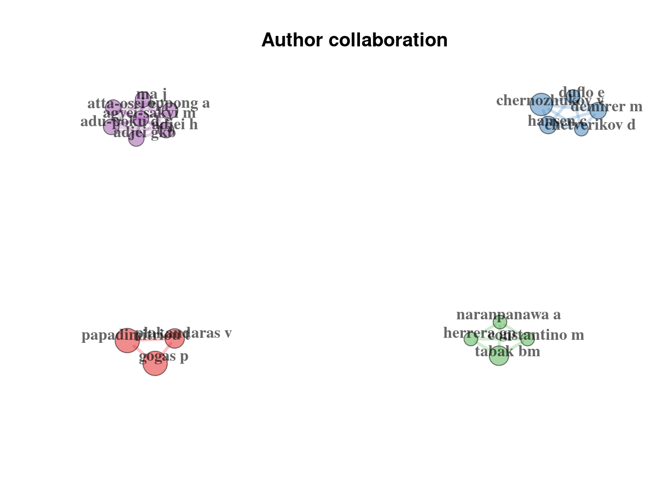
Here we can observe the interactions between authors, which are divided into four groups.
Alternatively, we can observe the institute interactions, because we have data on the authors affiliations:
# University network
uni_mat = db %>%
    biblioNetwork(
        analysis = "collaboration",
        network = "universities",
        sep = ";"
    ) %>%
    networkPlot(
        n = 30, Title = "University collaboration",
        type = "kamada", # "fruchterman", "kamada", "auto", "mds", "circle", "sphere",
        remove.isolates = TRUE,
        size = 10, size.cex = TRUE,
        edgesize = 3, labelsize = 1,
        weighted = TRUE,
        label.n = 15,
        remove.multiple = FALSE
    )
# University network
plot(uni_mat$graph)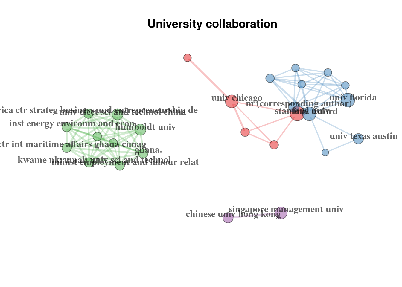
The correct functioning requires the citation information to be provided, meaning CR field should not be empty.↩︎